Self-play in reinforcement learning is a powerful yet tricky to use tool. While it is possible to learn effective policies with little human input, agents can get stuck in local optima and overfit to opponent’s policies. In this blog post I use (and extend) a recently developed metric for measuring overfitting in multi-agent reinforcement learning - joint policy correlation - to quantify the policy improvement from two simple modifications to vanilla self-play. The first improvement is early-stopping, a ubiquitous method from supervised learning where training is stopped before test loss starts to increase. The second improvement is pool-training, where the self-play opponent is randomly swapped out from a pool of opponent policies (that are being trained simultaneously). The combination of these two simple improvements yields a reduction in overfitting that is comparable to more complex methods.
Introduction
Self-play is a method of training RL algorithms where an agent repeatedly plays a game against itself and uses the experience generated to improve its policy. This requires relatively little human input as it’s possible to start with an untrained (i.e. completely random) agent that learns and explores the game from a blank slate.
The archetypal self-play success of recent years is AlphaGo (and its successors AlphaZero and MuZero) which was the first computer program to beat a human professional in the ancient game of Go in 2016. However self-play has seen good results as far back as 1992 when TD-Gammon achieved professional level play in Backgammon through temporal difference learning. Self-play has also achieved breakthrough successes in real-time-strategy video games such as Starcraft and Dota 2 which have much larger action spaces than chess or Go and are partially-observable to boot.
Relatively little work has been done on studying overfitting in (multiagent) reinforcement learning - something I attribute to the fact that most academic benchmarks, Atari being a prominent example, have no train/test distinction. A notable exception to this is “A Unified Game-Theoretic Approach to Multiagent Reinforcement Learning” ([Deepmind-MaRL] hereafter) which introduces a new metric, joint policy correlation (JPC), to quantify overfitting in multiagent RL and also a theoretically motivated algorithm, Deep Cognitive Hierarchies (DCH), to train agents with low JPC.
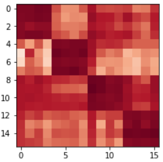
JPC is measured by constructing a JPC matrix - a square matrix of size D. To do this D instances of the same self-play experiment are run, differing only in the random seed. Each of the D experiments produces two policies \( (\pi^d_{1}, \pi^d_{2}) \). The value in row i and column j of the JPC matrix is the mean return (i.e. total undiscounted reward) over many episodes when player 1 uses policy \( \pi_{1}^{d_i} \) and player 2 uses policy \( \pi_{2}^{d_j} \). Entries on the diagonal represent the returns for policies that were trained together, i.e. a train-set performance metric and off-diagonal elements show returns for policies that were not trained together, i.e. a test-set performance metric. A particularly nice thing about this construction is its neither limited to 2-player games (just use an N-d JPC tensor) nor symmetrical games.
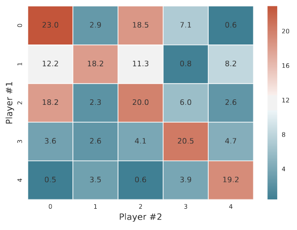
The authors define average proportional loss as \( R_{-} = (\bar{D} - \bar{O}) / \bar{D} \) where \(\bar{D}\) is the average value of the diagonals and \(\bar{O}\) is the average value of the off-diagonals entries and use this value as the primary performance criteria. However I’d argue that its much more important to look at the absolute magnitude of the off-diagonal reward as the key performance metric as a set of \(D\) random, untrained pairs of policies will result in a complete lack of overfitting (i.e. \(R_{-} = 0\) ) but also useless policies.
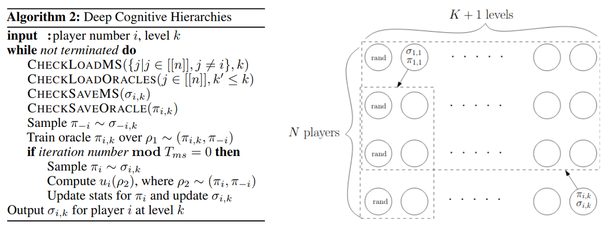
Like a lot of Deepmind’s work, DCH involves an inner and outer optimisation process. In DCH’s case the inner optimisation is self-play, training \(n\) oracle policies (for an \(n\) player game) in a multi-agent environment. The outer optimisation trains \(n\) players, which are just policies that operate at a higher level of abstraction. The oracle policies operate at the level of the environment, outputting an action and receiving rewards at each environment and are trained with deep reinforcement learning as standard. At each outer step the players simply choose one of the \(n\) oracle policies to play for them and receive reward equal to the total reward earned by that policy over a complete episode of the environment (against/with whatever policy the other player(s) selected).
Hence the players are in a multi-armed bandit where each arm of the bandit corresponds to the choice of inner policy. As the inner policies are constantly being trained the reward of each arm can change over time and the authors use an online-learning method (that I confess to not having digested enough to summarise) to determine the appropriate player policy based on the empirical payoff tensor i.e. the past rewards earnt by picking different arms.
So the Deep in Deep Cognitive Hierarchies comes from Deep RL used to train the oracle policies, the Cognitive part just sounds cool, where does the Hierarchies part come in? Actually theres a bit more to DCH, to use it one needs to choose a number of levels, \(K\), as a parameter. For an \(n\)-player game \(nK\) processes are started and each one trains a single oracle policy \(\pi_{i, k}\) and player \(j\) at level \(k’\) can choose not just from its oracle policies at its level but oracle policies at its level and all lower levels i.e. \(\pi_{j, k<=k’}\). The whole setup is parallelisable and each process saves its oracle policy to a central disk periodically. This means that each process uses slightly out-dated copies of other process’s policies but this is an intentional tradoff of accuracy for practical efficiency and scalability.
Method
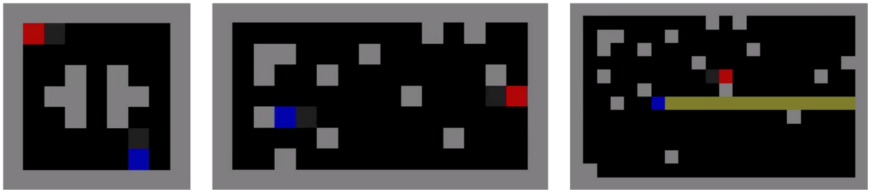
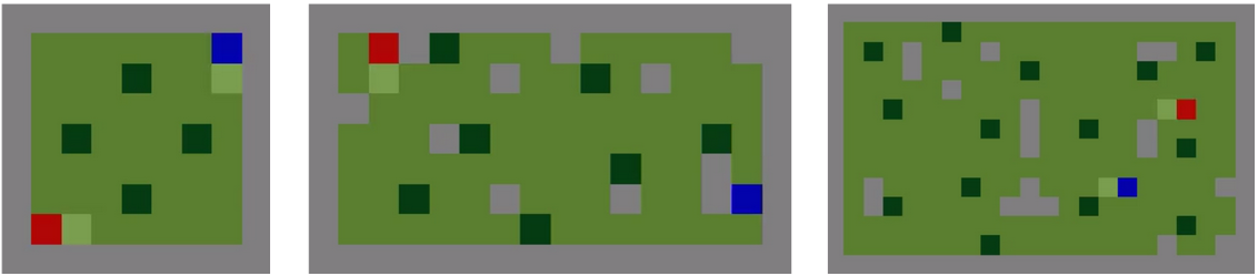
For this blog post I measured overfitting in two first-person, gridworld, multi-agent environments, one co-operative and one competitive. The experiments for each environment were repeated for 3 different “maps” with the same dynamics but different sizes and levels of partial observability.
The first environment is laser_tag which is a reproduction of the environment of the same name from “A Unified Game-Theoretic Approach to Multiagent Reinforcement Learning” . At the beginning of each episode each of the two agents start on a random spawn point. Agents are available to rotate, move in all 4 directions, fire an endless light-beam in their current facing direction and perform a no-op. If an agent is tagged by another agent’s light beam twice that agent is teleported to a random spawn point and the source agent is given 1 reward. Agents do not receive a negative reward for being tagged and all actions are executed simultaneously then resolved in a random order.
The second environment is harvest which has the same actions as laser_tag but the “fire” action is replaced with a “harvest” action. Plants (represented by a dark green square) are scattered throughout the environment and if both agents stand within 1 square of a fruit and simultaneously perform the “harvest” action then the fruit will disappear and both agents will receive 1 reward. Plants respawn at a fixed frequency that decreases with increased map size.
Both environments are implemented (see my earlier blog post) purely with vectorised matrix operations in PyTorch and hence can be run at high levels of batching on a GPU, the environment batch size used in this work is 128. The architecture of all agents is a 3 layer convolutional network with strides (2, 1, 1) and kernel sizes (4, 5, 3) followed by a flattening and Gated Recurrent Unit. All agents are trained using PPO with a learning rate of 5e-4, 128 step trajectories, entropy regularisation parameter 0.01, batch size of 32 and 9 epochs.
Results
Early stopping
In supervised learning it is typically observed that both train and test loss decrease early in training while later on test loss increases while train loss stagnates or decreases only slowly. Early stopping is a commonly applied form of regularisation in which training is stopped when test loss begins to increase. The same approach can be applied to non zero-sum multiagent games as well if we use diagonal and off-diagonal returns in place of train and test loss.
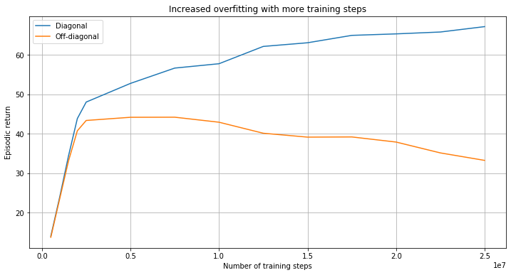
The figure below shows a typical example of a training run from this work (environment=harvest, map=small3). Note that the diagonal return increases monotonically with training whereas the off-diagonal return peaks much earlier in training, indicating that agents trained in this way increasingly overfit to each other’s behaviour with continued training.
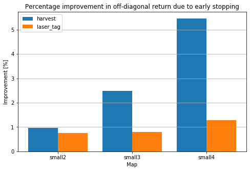
The figure below shows the percentage improvement in off-diagonal mean episodic return due to early stopping for all size (environment, map) combinations. Note that in order to reduce experimentation time I aimed to train policies until just after maximum off-diagonal reward. Hence these numbers could be boosted arbitrarily by say, training all policies for N times as many steps so the off-diagonal return would drop further.
Agent-pool training
The simplest and most obvious method to reduce the level of overfitting to a single self-play opponent is to not train against a single opponent but a pool of opponents, randomly swapping opponents in each episode. To maintain the same generality to non-symmetric games that DCH does I implemented agent pool training with separate pools for each player even though both of my 2-player environments are symmetric, this had some negative consequences (see Discussion).
The generalisation ability of agents trained by pool training can be assessed by examining a JPC matrix as before, however in the pool training case some off-diagonal entries can contain returns of two agents which have co-trained. Hence, I generalise JPC to block-diagonal JPC where diagonal (i.e. train) return becomes block-diagonal return which is the mean of block-diagonal entries with a block size of N-pool. Off-diagonal (i.e. test) return is simply the mean of entries not in the block diagonal.
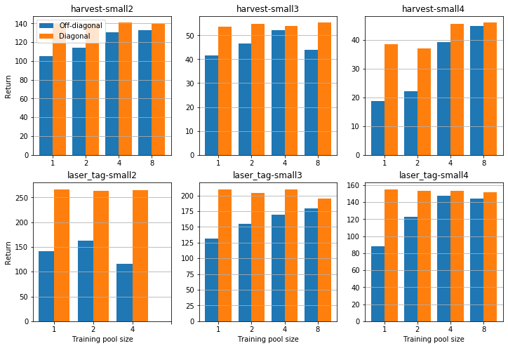
Each plot in the figure above shows the diagonal and off-diagonal reward for agents trained in different pool sizes. Note that the off-diagonal return increases with pool size in every case except laser_tag/small2. The diagonal reward stays roughly constant except for the interesting harvest/small4 case, as \(D\) and \(O\) both increase. Visual inspection of training runs shows that the reason is for this that the diversity of agents within a pool drives improved exploration. In a pool size of 1 a pair of agents typically converges into following a fixed route between 3 plants in the environment, these routes typically differ between training runs. In pool training agents have to learn to co-operate with agents that have learnt a different path between the plants, leveraging the exploration of other agents to reach a greater total number of plants.
 |  |
Discussion
[Deepmind-MaRL] give a single value of \( R_{-} \) for each training run and do not specify after how many training steps these values are measured. I’ve incorporated early stopping and taken my values of \( R_{-} \) at the number of training steps where the highest off-diagonal reward was reached and at the optimal pool size (8 for all env/map combinations except laser_tag/small2). The values of \( R_{-} \) for simple agent-pool training vs DCH are comparable and the two methods utilise a similar amount of compute as DCH training N=10 pairs of agents simultaneously. Agent-pool training has a lower “mental complexity” than DCH as it requires no lengthy game-theoretical justification, just application of the most obvious solution.
The exception is laser_tag/small2 where agent pairs consistently converge into a defender/attacker pattern where the defender agent remains stationary and waits for the attacker agent to approach. Defender/defender and attacker/attacker matchups result in weak performance as they result in both agents remaining stationary or both agents circling without scoring any points, respectively. The reason that this happens so consistently is that the agent pools for player 0 and player 1 are disjoint, imitating the setup in [Deepmind-MaRL], even though laser_tag is a symmetrical game player 0 and player 1 are identical. This means that once the agent pool for player 0/1 is filled with defenders and attackers respectively there will be no defender/defender or attacker/attacker matchups in training. Inspecting the policies throughout trainng reveals the sequence of steps that leads to this situation:
- Both agents start with random policies
- Either one of the agents learns to move towards the opponent and fire, becoming attacker-like
- The other agent responds by learning to return fire to the attacker without learning to move, as it doesn’t need to, becoming defender-like
- This problem persists in pool-training because as soon as one agent in the pool for player i becomes attacker-like the agents in the pool for player not-i are pressured to become defender like
This problem could be removed by using a single pool for all identical players. This issue is only problematic in the small2 map as there is line of sight between respawn points allowing defender-like policies to tag other agents without moving.
 |  |  |
The observation most surprising to me is that an agent, trained on a toy multi-agent task can fail to generalise when interacting with another agent trained on the same task with identical architecture and training parameters. The reduction in return can be >50% (harvest/small4). As the trend seems to be increased overfitting with increased complexity of the task I would expect more complex tasks to suffer even more from this problem. However this tentatively appears not to be the case as Open AI 5 can generalise to human teammates.
| Environment | Map | \( R_{-} \), this blog | \( R_{-} \), DCH |
|---|---|---|---|
laser_tag | small2 | 0.382 | 0.055 |
laser_tag | small3 | 0.083 | 0.082 |
laser_tag | small4 | 0.040 | 0.150 |
harvest | small2 | 0.070 | - |
harvest | small3 | 0.032 | - |
harvest | small4 | 0.138 | - |
Perhaps it’s the toy nature of these tasks that lend themselves so well to overfitting. The agents are not learning a generalised policy that a human might but instead memorising more or less fixed sequences of actions. This fits with my intuition that neural networks will learn the easiest solution to a problem, not the most generalisable. The reason that pool-training and DCH train better policies is that they make the tasks harder as agents have to be successful against multiple opponents. This produces better experience data and lets these methods leverage the bitter lesson (i.e. more data and more compute always wins in the end) more effectively and produce better policies).