In this blog post I’ll guide you through my most recent project, which combines two things I find fascinating — computer games and machine learning. For quite a while now I’ve wanted to get to grips with deep reinforcement learning and I thought there is no better way than to do my own project. To that end I implemented the classic mobile game “Snake” in PyTorch and trained a reinforcement learning algorithm to play it. This post is divided into three parts.
- A massively parallel vectorized implementation of the Snake game
- An explanation of Advantage Actor-Critic (A2C)
- Results: analysing the behaviour of different agents
Code for this project is available at [https://github.com/oscarknagg/wurm/tree/medium-article-1]
Snake - vectorized
For all it’s impressive achievements, deep reinforcement learning is very slow. Incredible results have been achieved in complex games like DotA 2 and Starcraft but these have taken 1000s of years of gameplay. In fact even the work that sparked the current wave of interest in deep reinforcement learning, i.e. learning to play Atari games, required weeks of gameplay and 100s of millions of frames for each game.
A lot of research since then has been done towards speeding up deep reinforcement learning, both in terms of wall clock time by parallelisation and improved implementation and also in terms of sample efficiency. Many state of the art reinforcement learning algorithms are trained in multiple copies of an environment simultaneously, typically one per CPU core. This yields a roughly linear speed up in how fast you can generate gameplay experience with more CPU cores.
So in order to experiment with deep reinforcement learning you had better have either a lot of computational resources, a very fast/parallel environment or be willing to wait a long time. Since I don’t have access to a large cluster and want to see results fast I decided to create a vectorized implementation of Snake which can achieve a much greater level of parallelisation than the number of CPU cores.
What is vectorization?
Vectorization is a form of single instruction, multiple data (SIMD) parallelism. For those of you who are Python programmers this is the reason that numpy operations can often be orders of magnitude faster than explicit for-loops that perform the same calculations.
Essentially, vectorization is possible because if a processor can perform operations on, say, 256 bits of data in a singe clock cycle and your program’s real numbers are 32 bit single precision numbers then you can pack 8 of these numbers into 256 bits and perform 8 operations with each clock cycle. So if a program is clever enough to schedule instructions such that there are always 8 operands in place at the right time it should be able to achieve, in theory, an 8x speedup over executing instructions on one piece of data at a time.
Implementation: Representing the environment
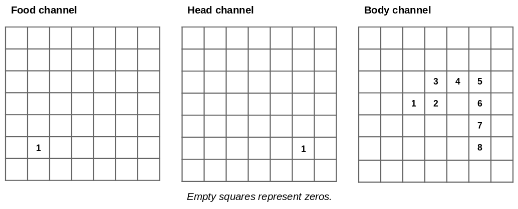
The key idea is to represent the full state of the environment as a single tensor. In fact multiple environments are represented as a single 4d tensor in the same way that a batch of images is represented. In the case of Snake each image/environment has three channels: one for food objects, one for snake heads and one for snake bodies as shown above. Doing this lets us leverage the many features and optimizations that PyTorch already has for manipulating this kind of data.

Implementation: Moving the snake
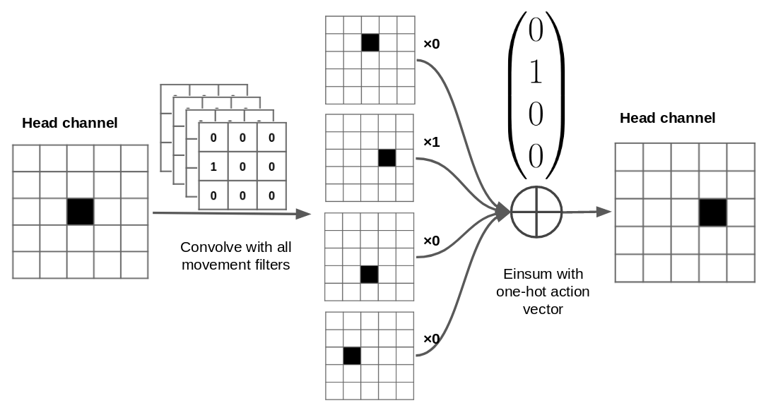
So now that we have a way of representing the game environment we need to implement the gameplay using only vectorized tensor operations. The first trick is that we can move the position of all the snake heads in every environment by applying a 2D convolution with a hand crafted filter to the head channel of our environment tensor.
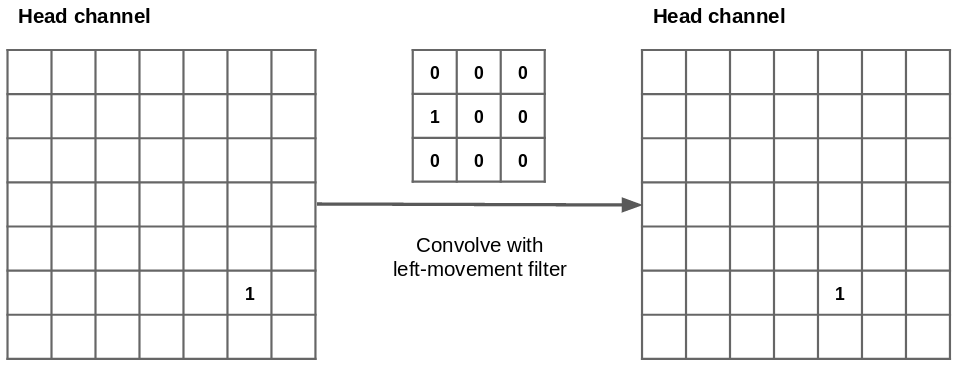
However PyTorch only lets us apply the same convolutional filter to the whole batch but we need to be able to take a different action in each environment. Hence I apply a second trick to work around this limitation. First apply a convolution with 4 output channels (1 for every direction of movement) to each environment then use the very useful torch.einsum to “select” the correct action using a one-hot vector of actions. I’d highly recommend reading this article for a very good introduction to Einstein summation and its uses in NumPy/PyTorch/Tensorflow.
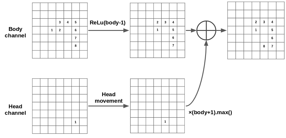
Now that we moved the head we need to move the body. Firstly we move the tail (i.e. the 1 position on the body) forwards by subtracting 1 from all body locations then applying the ReLu function to keep the other elements above 0. Secondly we make a copy of the head channel, multiply it by the maximum body value plus 1. We then add this copy to the head channel which creates a new front position for the body (position 8 in the diagram).
Environment simulation speed
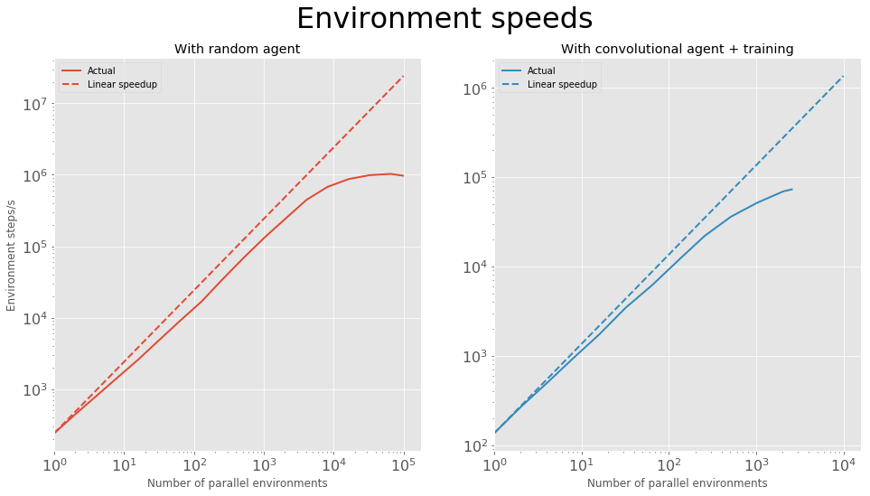
There’s a bit more logic required such as checking for collisions and food collection, resetting environments after death and checking snakes aren’t trying to move backwards — it was very fun thinking of ways to implement all this in a way that is vectorized across multiple environments. The end result of all this optimisation is shown in the plots below. With a single 1080Ti and an environment of size 9 I can run a maximum of just over a million steps per second with a random agent and just over 70,000 steps/s while training a convolutional agent with A2C (using the same hyperparameters as for the later results).
Advantage actor-critic (A2C)
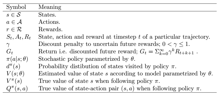
In this section I assume your familiar with the basic terminology of reinforcement learning e.g. value function, policy, rewards, returns etc.
The idea behind the actor-critic algorithm is simple. You train an actor network to map from observed states to a probability distribution over actions i.e. the policy. The aim of this network is to learn the best actions to take in a particular state.
At the same time you also train a critic network that maps from states to their expected value i.e. the sum of future rewards expected after being in this state. The aim of this network is to learn how desirable it is to be in a particular state. This network also stabilizes the learning of the policy network by providing a baseline value for states as we’ll see later.
Value function learning
The loss of the value function is the squared difference between the predicted value of a particular state and the actual (discounted) return generated from that state. Hence value function learning is a regression problem.
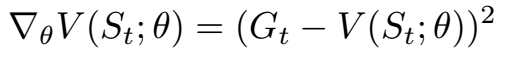
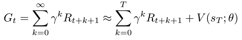
In practice, calculating the true return for a particular state requires having the trajectory starting from that state until the end of time, or at least until the death of the agent. Due to finite computational resources we calculate the return from a trajectory of a fixed finite length, T, and use bootstrapping to estimate the distant returns after the final trajectory state. Bootstrapping is means we replace the final part of the sum with the predicted value of the final state in the trajectory — the predictions of the model are used as its targets.
Policy learning
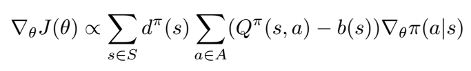
There is an important result in the field of reinforcement learning known as the Policy Gradient Theorem. This states that for a parametrised policy, (e.g. a neural network mapping from states to actions) their exists a gradient on the parameters that leads to an increase in the performance of the policy, on average. The performance of the policy is defined as the expected value of states over the distribution of states visited by that policy, as shown below.
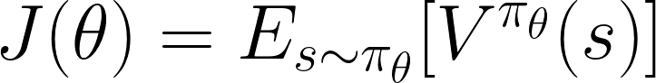
This is actually a more surprising result than it first seem. Given a particular state, computing the effect of changing the policy parameters on the actions and hence reward is relatively straightforward. However, we are interested in the expectation of the reward across the distribution of states visited by the policy, which will also change with the policy parameters. The effect of changing the policy on the distribution of states is usually unknown. Hence it is quite remarkable that we can calculate the gradient of the performance with respect to the policy parameters when the performance depends on the unknown effect of policy changes on the state distribution.
Shown below is the general form of the policy gradient algorithm. A proof and a complete discussion of this theorem is out of scope but I would recommend Chapter 13 of “Reinforcement Learning: An introduction” by Sutton and Barto if you’re interested in digging deeper.

With a little bit of math we can write this as an expectation over a states and actions visited by our policy.
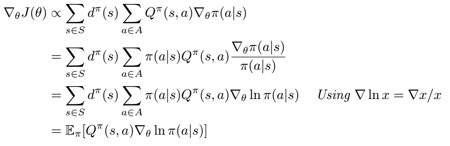
This expression is a little easier to get an intuition for. The first part in the expectation is the Q-values of state-action pairs seen by the policy i.e. a performance measure. The second part is the gradient that increases the log-probability of a particular action. Intuitively the overall policy gradient is the expectation of individual gradients that increase the probability of high reward actions. Conversely, if Q(s, a) is negative (i.e. bad actions) then individual gradients must decrease the probabilities of these actions.
An important insight into the policy gradient theorem as stated earlier is that it doesn’t change if an arbitrary action-independent baseline b(s) is added to the Q function.
Adding this baseline function introduces a new term to the policy gradient, which given that is action-independent, is always equal to 0.
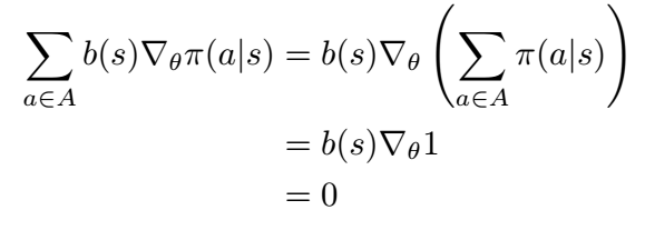
Although adding a baseline doesn’t affect the expectation of the policy gradient it does affect its variance, so a well chosen baseline can speed up the learning of a good policy.
The baseline that is chosen in A2C is the advantage function (hence advantage actor-critic). This quantifies how much better a particular state-action pair is when compared to the average action from that state.
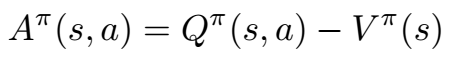
Based on this expression it looks like we will need to learn another network to approximate Q(s, a). However we can rewrite this in a much simpler way.

We can do this because the definition of the Q function for a particular policy is the reward from action a in state s plus expected return from following that policy for the rest of the episode. Hence the final advantage actor-critic gradient is as follows.

Overall algorithm
Now that I’ve sketched out the theoretical underpinnings of A2C its time to see the full algorithm. All we need to obtain an incremental improvement of our policy is a way to obtain samples such that the expectation of the gradient of those sample is proportional to the expression above. This can be achieved very simply by recording trajectories of experience generated by our policy. In order to accelerate this we can run multiple copies of our policy in parallel on the same environment to generate experience faster.
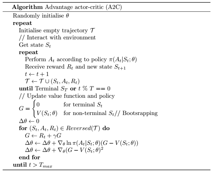
This is the synchronous version of the famous asynchronous advantage actor-critic algorithm (A3C). The difference is that in A3C the parameter updates are calculated in many worker threads separately and used to update a master network which the other threads periodically synchronize with. In batched A2C the experience from all workers is combined periodically to update the master network.
The reason that A3C is asynchronous is so that differences in environment speeds in different threads don’t slow each other down. However in my snake environment the environment speeds are always exactly equal by design so a synchronous version of the algorithm makes more sense.
Results
Now that I’ve described the implementation and theory its time to learn to play snake! In my experiments I compare the performance of three different architectures, pictured below.
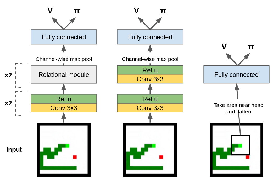
The first agent (left) is a smaller version of the agent from Deepmind’s “Deep reinforcement learning with relational inductive biases” paper. This agent contains a “relational module” which is essentially the self-attention mechanism from a transformer model applied to a 2D image. After this we apply channel-wise max pooling and a single fully connected layer before the value and policy outputs. For comparison I also implemented a convolutional agent (middle) which is otherwise the same except the relational modules are replaced with more convolutional layers.
As a dark-horse competitor I introduced a simpler, purely feedforward agent (right) which only takes as input the local area around the head of the snake, making the environment partially observable. The input observation is flattened and passed through two feedforward layers. The value and policy outputs are linear projections of the final activations, just as the other two agents.
All 3 agents were trained 5 times for 50 million steps on a size 9 environment. The training curves with 1 standard deviation are shown below.
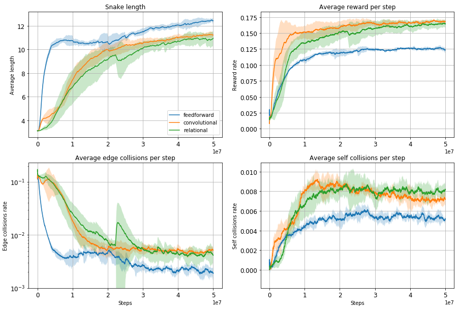
Surprisingly the feedforward agent that only has partial observability of the environment performs very well, achieving the highest average size of all agents. It also learns the quickest, probably due to having the smallest observation space. As you can see from the GIF below it has learnt to avoid the drawback of only having limited visibility by circling the environment so that all of it eventually passes into view. This allows it to find the rewards scattered around the environment but not as efficiently as the convolutional and relational agents.

The other agents move more or less directly towards the rewards but also have a tendency to make some stupid mistakes, reflected in the fairly high edge collision rate compared to the feedforward agent. Its also interesting to note that for this task the relational agent performs no better than the convolutional agent. I hypothesis that the snake environment is too simple for the inductive biases incorporated into the relational module to be useful. The task on which Deepmind benchmarked the relational agent involved collecting multiple keys for multiple boxes in order to collect a final large reward — much more complex than snake!

Transferring to a larger environment
As a bonus experiment I decided to see what would happen if I transferred the agents from the small size 9 environment to a larger size 15 environment. I evaluated the performance of 5 instances of each type of agent for 1 million steps on the larger environment, with no further training.
![]()
This table shows a huge variation in transfer performance between agent types and even within particular training runs. The convolutional agents generalise very well, achieving a large average size and high reward rate. In fact the convolutional agents perform better than the same agents trained from scratch in the larger environment. I believe this is because rewards are sparser in the larger environment and so learning is slowed down significantly in the larger environment.
Some fairly clever behaviour can be observed. At large snake sizes the convolutional agent will sometimes be seen to perform a “coiling” maneuver while it waits for its tail to move out of the way.

The limited visibility agent continues the same behaviour of circling around the edge of the environment. This can perform quite well until a food pellet spawns in the center of environment which the agent is not able to observe and from this point on the agent collects no more reward. This is consistent with the large size and small reward rate in the table above.
![]()
The performance of the relational agent is unstable to say the least. In some runs it will perform quite well, while in others it will die almost immediately or get stuck in a loop.
![]()
Conclusion
In this project I’ve seen firsthand the slowness of deep reinforcement learning and come up with a neat, if brute-force way of getting around it. I’ve also experienced the brittle nature of deep RL by observing failed transfer between quite similar environments.
In future work I’d like to implement more gridworld games in order to investigate transfer learning between games. Or perhaps I will implement a multi-agent snake environment in order to answer OpenAI’s “Slitherin’” request for research.